| " " |
|
| Facilities Research Publications Patents Astronomy Software SSC Observatories Contact Us | ||||||
Ground Based Determination of Meteor Trajectories and Satellite Orbits
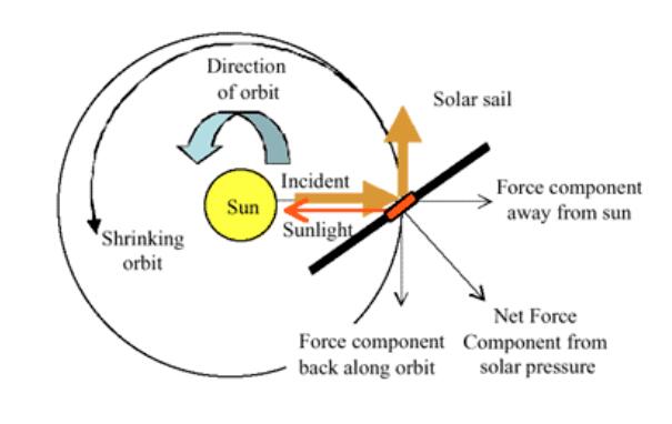
My work on the development of methods to measure the trajectories of meteors and satellite orbits originated several years ago from a collaboration with NASA's MSFC on the ill fated Cosmos I Solar Sail Program. For years NASA has been exploring alternate propulsion technology that offer larger payload, or more efficient propulsion than chemical rockets to take us far outside of Earth's orbit. Among the technologies investigated are nuclear thermal propulsion, nuclear ion propulsion, photo-voltaic ion propulsion and solar sails. Several spacecraft, both commercial and government sponsored have demonstrated the viability of ion propulsion. Among the most notably are the Dawn and Deep Space-1 missions to asteroids that have employed ion propulsion. Solar sails have yet to been similarly demonstrated in space. 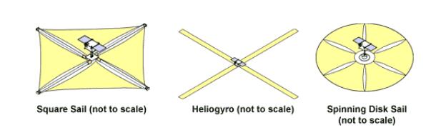 Solar Sails Solar sail technology has languished in the face of shrinking NASA Science and technology budgets and through launch misfortunes. In June2005 the Planetary Society tried to send Cosmos-1, an early prototype of a solar sail on a flight on a Russian Volna rocket. This was the mission in which I first became involved, but the spacecraft stayed attached to the rocket and did not deploy properly after from a submarine in the Barents Sea and crashed into the water. The experimental spacecraft was supposed to orbit Earth and raise its altitude solely using sunlight. 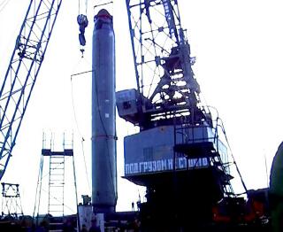  Volna Launch Vehicle and Submarine Launch Platform Thrust Determination A fundamental question was how to verifying the performance of the solar sail as a propulsion system. The resultant thrust produced by a solar sail is a function of many variables that are difficult to measure on the ground or predict from analysis. The parameters can be loosely grouped into two categories:
 Two approaches may be used to estimate thrust performance - indirect methods and direct methods. Indirect methods utilize ground tracking station data and Global Positioning System (GPS) measurements to determine the sail's orbit from which the thrust profile can be estimated. Orbit determination is the process whereby the spacecraft position and/or velocity is measured from Earth or other spacecraft. Direct methods utilize accelerometers aboard the spacecraft to measure the thrust performance. Direct measurement instrumentation adds significant cost, weight, and complexity to solar sail missions. As the weight increases, not only do the launch vehicle requirements escalate, but the resultant acceleration for a given propulsive input becomes smaller and harder to measure. Ground Based Thrust Determination In an effort to support these missions I was enlisted to develop methods that interested amateur astronomers and students could employ to make ground based measures to assist in determining the generated thrust. The basic idea was to extract astrometric data and visual magnitude data from ground based observers. Astrometric data is typically used to estimate the six constant Keplerian elements of the satellite In the case of solar sails, the Keplerian elements are functions of time. Hence, the aggregation of astrometric data is used to reconstruct the trajectory and estimate the thrust vector time history. Despite the fact that COSMOS-1 and NanoSat both failed to reach orbit, the developed methods apply equally well to other satellites and can be adapted to measure the entry trajectory, velocity and mass of meteors. For that reason, and in hopes that future solar sail tests will eventually reach orbit, I am summarizing the developed methods below. Observational Methods Several methods offer promise for the determination of the orbital elements. Each method is summarized in terms of the equipment and level of participation that might be required, organizational structures necessary and methods for mobilizing the required cadre of observers. I propose that these methods can be used to demonstrate the concept using various candidate objects such as the International Space Station. Method 1: Still Photography, Multi-Observer This method employs multiple geographically separated observers with still cameras capable of 5 second to 60 second exposures. Requirements:
 Observational Procedure Each film camera observer is instructed to take one daylight exposure to mark the start of roll and framing interval, and a second of a cue card containing the observer's name and the roll index number. The observers then take 15 second exposures of the satellite on the start of each minute and half minute during their passes. The film is subsequently processed to negatives. The negative and the observing journal page for that roll are submitted to the data reduction team. Users of digital still cameras can simply save their images in any uncompressed format, TIFF being the recommended standard, and can be transmitted on digital archival media to the data reduction team. Data Reduction and Analysis These images, taken with a normal 50mm lens will cover a field of view of approximately 45 degrees. The satellite should have transited about 10 degrees of the field. The exact start and end points of the arc can be determined from the image. Typical 35mm film, scanned at 2400dpi will resolve positions to about 1 to 2 arc minute accuracy. The background star field and local sidereal time and geodesy together will allow the satellite's azimuth and altitude to be solved. For more precise calculations atmospheric refraction can be used in the solutions. Off the shelf astrometric software such as "ASTROMET" can perform these reduction or IRAF scripts can be generated relatively easily. With this technique a moderate elevation pass (say 30 degrees for both observers) should allow observers on a 50 km baseline to locate the satellite to within a 15km radius circle of error. The time standard is the critical value. If timing can be held to within +/- 100msec the error circles diameter drops to 3 km. Method 2: Still Photography, Multi-Exposure This method requires only a single observer, but more sophisticated math. The idea is that the observer makes photos as in the multi-observer method. The data reduction team computes the precise Az, El and Time of the start and end point of each track on several images from the same pass. To the first order, these passes are Keplarian orbits precessed by the Earth's gravitation field. Using an interative method one can compute a least squares fit of the [Az, El, Time] observations to adjust to the initial NASA two-line elements to best match the observed pass. The most interesting method for adjusting the two-line elements is to treat the drag term as a vector rather than a scalar. By allowing it to have both a direction relative to the direction of motion, rather than treating it as a scalar against the direction of the motion, one effectively models the sum of drag and acceleration resulting from the sail. By adjusting only this quantity and fitting the observations one directly solves for the acceleration of the sail. It is a simple process to use the elapsed time since the ephemeris time, and with knowledge of the spacecraft mass, determine the mean force vector generated by the sail. Any earth orbit prediction program can of being modified to make this calculation. Distribution of this program to participants allows observers to perform their own analysis, provided they have a means:
Method 3: CCD Multi-Observer This method is similar in philosophy to the Photographic Multi-Observer Method, but instead of film this method utilizes an integrating CCD imager with short focal length lenses mounted upon a tracking telescopes. Requirements:
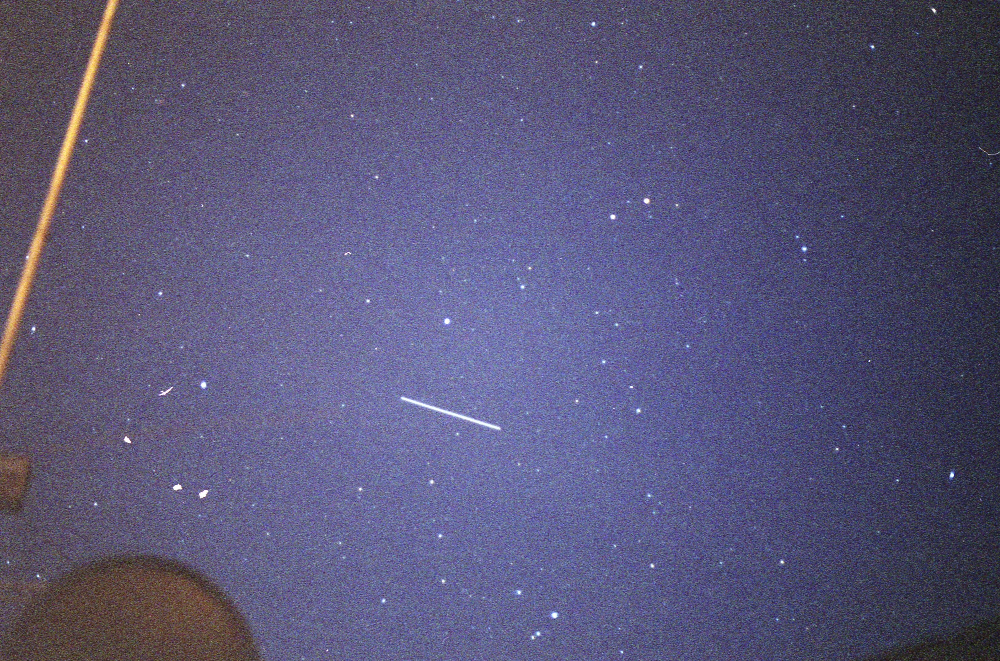
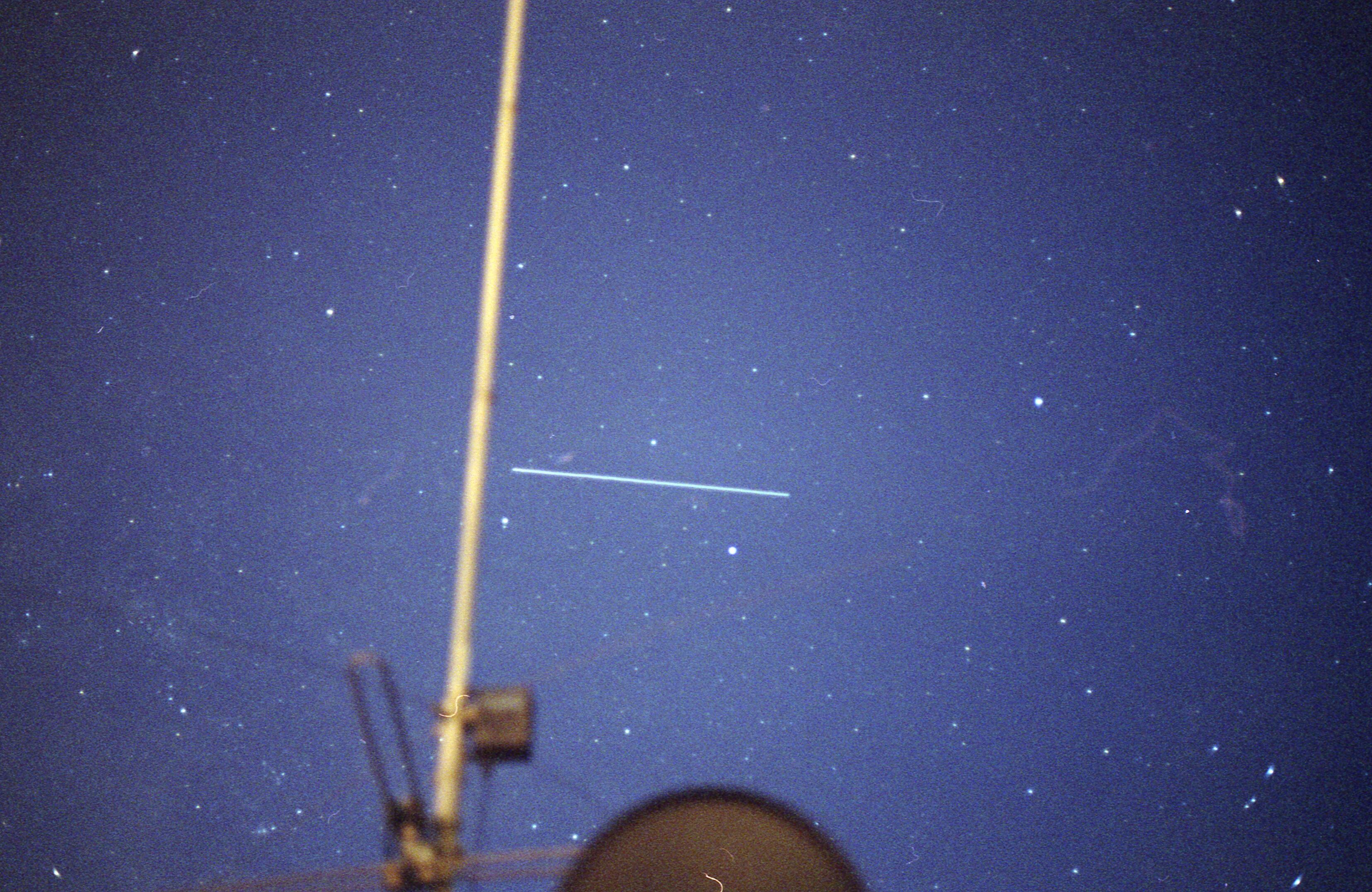
Satellite Pass 2/20/2006 Observational Procedure: Each observer is to slew their telescopes to the center of the predicted satellite pass. Prior to the pass, the observer will make a long duration exposure of the field of view, assuring that at least 10 stars of sufficient S/N ratio are imaged to ensure good astrometry of the images. During the pass, the observer will take a series of images of approximately 1 second duration during the pass until the satellite has transited the field. Observers should submit these images in FITS format with their observing journals on archival media to the data reduction team. Among the challenges of this method is the recording of the image time with very high accuracy. Provided that the PC clock is synchronized with the NIST time server, it should be possible to get +/- 0.1 second accuracy for exposure times. Data Reduction: As with the Photo-Multi-Observer method, astrometry is performed on images and the potential accuracy of these measurements is again time limited, but can be within +/- 3km. Method 4: CCD Multi-Pass This method, uses the same procedures as the CCD Mulit-Observer method, but measure the satellite position on successive passes. The same software and methodology as described for the Photo Multi-Exposure method can be used to solve for orbital acceleration. Experimental Procedure Validation I performed a series of tests to validate the experimental methods proposed above. To validate our method, I have been applying the proposed photographic and CCD imaging methods to bright satellites. The imaging targets have been satellites making passes with apparent magnitudes of 2.5 brighter. Targets have included ISS, HST, TRMM and serendipitous targets occurring during other CCD imaging projects. I have verified that satellites are easily photographed from suburban environments with the proposed setup. Even in the presence of significant light pollution, both the track and enough background stars are detectable to assure accurate astrometry. Analysis of the image in Figure 7, scanned at 2400 dpi, yielded a plate scale of 44.2"/pixel. FWHM of stars in the image averaged 7.8 pixels. This indicates a psf of 5.75' 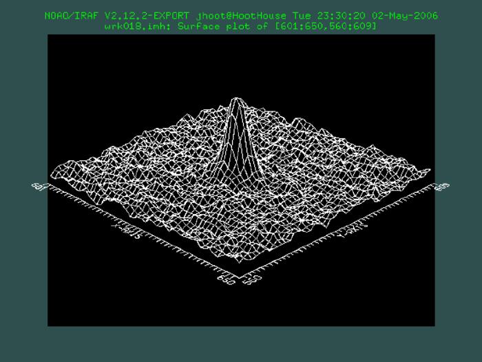
Typical 35mm Point Spread Profile at FL=50mmm Performing precise astrometry on wide field images proved a challenge. It could not be peformed with Astrometrica. The latest generation of the program is optimized for deep field minor planet work. As such, it uses USNO A.1, USNO A.2 and USNO B catalogs that do not include bright stars. Reversion to the older DOS based program succeeded in working with GSC 1.1 and ACT-GSC catalogs, but did not provide reasonable fits. 
Mean FWHM = 4.98pix Star FWHM=4.42pix Trailing ~ 0.61pix There are several factors that make phtotgraphic plate solutions challenging. Firstly, the fields themselves are very large and the pixel scale, at 44", is atypical for most astronomy. The second challenge is that wide field photographic lenses suffer from not only field curveture, but also from barrel distortions and astigmatisms as a result of their design for wide fields of view. Additionaly, the film scanning process can introduce additional distortions, notably skew. Finally, images taken in ALT-AZ with tripods always contain significant field rotations. These higher order corrections require more complex fitting than typical second order plate scale solutions. 
IRAF Plate Scale Solutions After looking into several alternatives, acceptable results were obtained using IRAF, now available running in native mode under Windows using the Cygwin library. Using 4th order plates solution polynomials, fits were obtained with residuals compatible with PSF of the plates. The 1 sigma RA error was 3.4' and the Declination one sigma error was 5.4'. Both are smaller than the PSF of the image. A script to automate the IRAF fitting routine is under development.
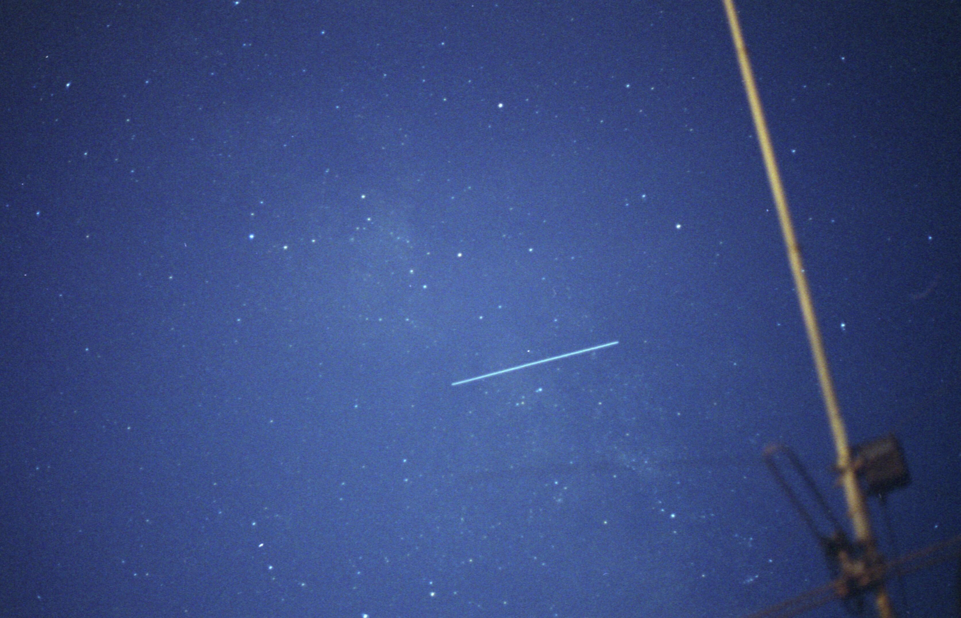
Satellite Time Lapse 2/20/2006 Similarly, wide field CCD images have proved the feasibility of their use. The image in Figure above was a 2 second exposure from a time lapse series that was produced during Mar's recent occultation of SAO76327. This 2 second exposure, and those bounding it, show the passage of a high inclination angle satellite through the frame. Analysis of the image show a plate scale of 42.414"/pixel and a FWHM of 3.6, yielding a PSF of 2.55'. This would indicate that short exposure, wide field CCD images should be able to provide about twice the positional accuracy of photography with comparable time resolution. With computer triggering of exposures and precision timing, even better results should be obtainable. Furthermore, flatter fields should also lead to better astrometry from all digital images. Conslusion These results have convinced me that the photographic methods are viable within the error ranges projected. These methods will reach the broadest audience of potential participants. The growing affordablity of capable digital cameras should make these methods even easier to achive. I am now in the process of taking further imagery and modifying SSC orbital prediction software to solve for satellite acceleration and orbits and to compute meteor entry trajectories.
|
||||||
|
|||